Singular value decomposition.

A powerful mathematical tool that arises from linear algebra is the “dimension reduction” method using the so-called singular value decomposition (SVD). This example is written in a tutorial style.

Matlab/Octave

In this set of exercises you will be using either Matlab or its libre counterpart Octave. It is advised to open a script file (File -> open -> create a script), and code there. If you run the code by pressing the “run” button (play icon). You can inspect the declared variables in the command-line section. This document will involve some coding, but I hope you will be able to follow the code snippets in this document. You may copy/paste and extend them.

Data in a square matrix

We can store all kinds of information in columns and concatenate columns to form a data matrix. We start by considering an artificial example: A researcher in biomedical engineering analyses data from $n$ patients. It so happens to be that he/she is interested in $n$ quantities regarding these patients. We illustrate the first patient’s column vector $\mathbf{p}_1$.

$$\mathbf{p}_1 = \begin{pmatrix} \text{Age: 45 years} \\ \text{Length: 180 cm} \\ \text{Aortic diameter: 2.2 cm} \end{pmatrix}$$

For 3 patients, we can place all the data in a matrix $A$, The rows imply the meaning and units.

$$A = \begin{pmatrix}45 & 40 & 55 \\ 180 & 170 & 170 \\ 2.2 & 2.3 & 2.1 \end{pmatrix}$$

This matrix maybe diagonalizable (why?). We can use Octave/Matlab to quickly find its eigen values and eigen vectors:

% Initialize matrix
A = [[45, 40, 50],
    [180, 172, 173],
    [2.2 , 2.3 , 2.1]];
% Compute eigen vectors and eigen values
[V, l] = eig(A);

1) Using the code below, verify that V and l are the “eigen decomposition” of $A = VlV^{-1}$. Hint: use inv(A) to find the inverse of a matrix A.

% Compute the reconstructed matrix `Ar` using the eigen decomposition
Ar = V*l*inv(V); 

2) Using the code below, verify that the eigen vectors are normalized

% Lets have a look at the first eigen vector
eig1 = A(:,1); 
% We can square the components and sum them to get the squared length
% Mind the dot in the element-wise square operator `.^2`. 
leig1 = sum(eig1.^2); 

From inspection of the matrix l, the matrix $A$ has three distinct (real!) eigen values, from large to small:

$$\lambda_1 = 216.85..., \lambda_2 = 1.55..., \lambda_3 = 0.06895$$

It appears that $\Lambda_1$ is much larger than the others. Imagine if we would set all values in the diagonal matrix (l) to zero, except for $\lambda_1$. We can call this a “low rank approximation” of the original matrix.

% Row-rank approximate diagonal matrix
l_lr = zeros(3,3);
l_lr(1,1) = l(1,1);

Instead of using the original decomposition ($A = VlV^{-1}$), we can attempt a low-rank approximation of the data set.

% Low rank approximation of A
A_lr = ...%fill in

Using the rules of matrix multiplication, we can see that the second and third column of V do not contribute to this product. Similarly, the second and third row of $V^{-1}$ play no role in this approximation. As such, we can approximate the matrix $A$, using fewer data. The approximation requires 3 + 1 + 3 = 7 non-zero data entries, instead of the original 9 (3 times 3). This is a “lossy” data compression method, as we are not able to reconstruct the original data matrix exactly.

3) Rewrite the low-rank approximation as a column vector - row vector multiplication.

4) Have a look at the component values in the first eigen vector (associated with $\lambda_1$). What do these numbers tell you about an “Eigen person”?

Notice that we could make a better approximation if we would include the second largest eigen value, and its associated column and row in $V$ and $V^{-1}$, respectively.

Data compression in a rectangular matrix

Grey-scale image data consist of a grey-scale value for each pixel in the image. We can import an image and convert it to a grey-scale matrix using the following code in Octave/Matlab. (replace the link with a non-square (moderately sized) image/photo that you like).

% Load an image via a path or the internet
[Image,b] = imread ("https://assets.w3.tue.nl/w/fileadmin/_processed_/\
3/f/csm_Gemini_zuidzijde_396-fr2-a0002_web_0b845bfc46.jpg");
% The color Image is now represented as a `m x n x 3` matrix.
% We should average over the 3rd dimension (RGB-values) to obtain a grey-scale image
grey = mean(Image, 3); 
% Inspect the grey-scale image using,
size (grey)
imshow (grey, b);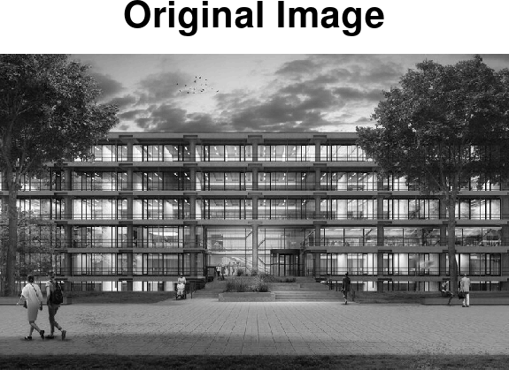

Since the image it not square, we cannot readily apply the eigen-decomposition method above. However, $A^TA$ and $AA^T$ are square, and these will appear to encode (some) of the data of our grey-scale image.

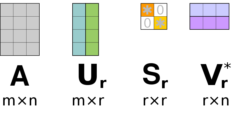
We will strive to find the matrices $U, S, V$ that decompose a matrix $A$, according to.

$$A = USV^{T}.$$

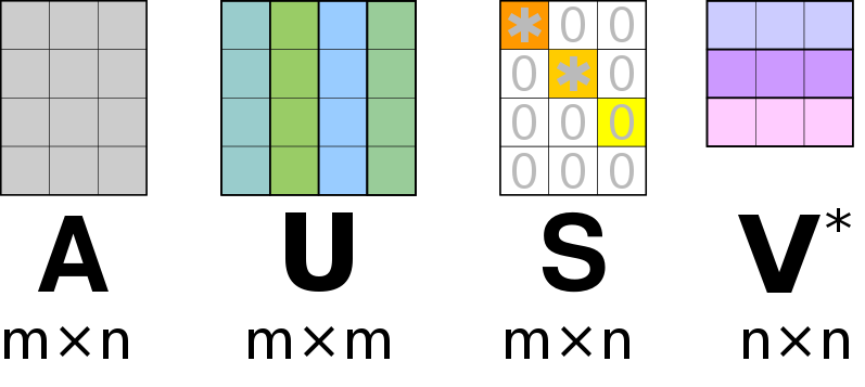
Similar to the eigen-value decomposition $S$ will be a diagonal matrix. For $A$ an $m \times n$ matrix, the matrix $U$ will be of size $m \times m$, the diagonal matrix $S$ will be of size $m \times n$ and $V$ will be a $n \times n$ matrix. For an SVD ($A = USV^T$) decomposition, we dictate that the columns of $U$ and $V$ must be normalized, this ensures that the diagonal entries of $S$ are the “weights” associated with the corresponding columns of $U$ and $V$. Furthermore, the ansatz is that the columns in $U$ and $V$ are orthogonal. An auxiliary theorem (not part of this course) states that for an orthonormal matrix ($N$), its inverse is equal to its transpose;

$$N^{T} = N^{-1}.$$

Lets derive an expression that relates $A$, $S$ and $U$.

$$A = USV^T,$$ $$AA^{T} = USV^T(USV^T)^T,$$ $$AA^{T} = USV^TVS^TU^T,$$ $$AA^{T} = USS^TU^T,$$ $$AA^{T}U = USS^T.$$

And analogous,

5) Proof that $A^TAV = V S^TS$

We can see that the columns of $U$ and $V$ are the eigen vectors of $AA^T$ and $A^TA$, respectively, with the eigen values the associated entries of the diagonal square matrices $SS^T$ and $S^TS$, respectively.

Our ansatz that the columns of $U$ and $V$ are orthogonal is hereby closed. This is rooted in an auxiliary theorem (not part of this course) that states that the distinct eigen vectors of a symmetric matrix ($M$) are orthogonal.

6) Show that $A^TA$ and $AA^T$ are symmetric matrices.

A failing attempt

The next computer coding is related to finding the eigen values and eigen vectors for $A^TA$ and $AA^T$. We can use Octave’s eig function.

% Compute the two square matrices
AAT = grey*transpose(grey);
ATA = transpose(grey)*grey;
[U, STS] = eig(AAT)
[V, SST] = eig(ATA) 

7) Inspect the sizes of the matrices U, V, STS and SST

8) Inspect the eigenvalues using,

plot (abs(diag(STS)))
hold on
plot (diag(SST))
set(gca, 'YScale', 'log')
hold off; 

We should ensure that the eigen values appear in descending order and also reorder the eigen vectors accordingly.

% Sort eigen values and vectors
[sst, idx] = sort(diag(SST), "descend");
Us = U(:,idx);
[sts, idx] = sort(diag(STS), "descend");
Vs = V(:,idx);

9) Compare the eigen values sst and sts

Now we should compute $S$.

10) Show that the diagonal entries of $S$ (i.e. the singular values) are the square roots of the eigen values stores in sts and/or sst.

We can now compute $S$,

% Compute the singular-value diagonal m x n matrix (S)
s = sqrt(sst);
sg = size(grey);
S = diag(s, sg(1), sg(2));

We are now ready to test our singular value decomposition

11) Inspect the sizes of U, S, V, the singular values, and, using the code below, verify the decomposition.

gr = U*S*transpose(V); 
imshow (gr, []);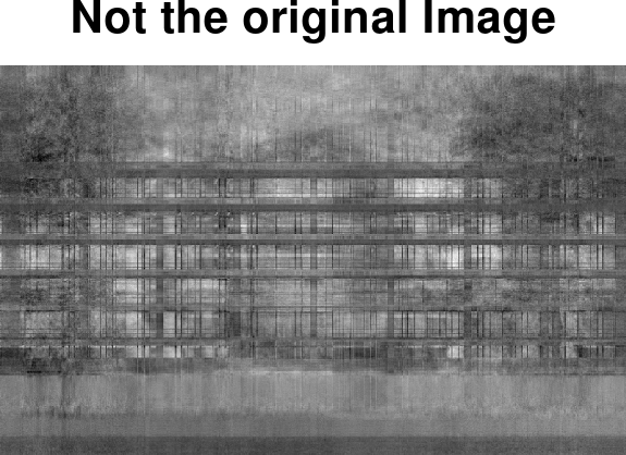

A successful decomposition

Indeed, when we discovered that both $AA^{T}U = USS^T$ and $A^TAV = V S^TS$, we have wrongly assumed that these equations ensure that the original decomposition $A = USV^T$ is automatically satisfied. This would have worked if the singular value decomposition is unique. But there may exist many matrices ($B$) that are smilar to $A$ in the sense that $BB^{T} = AA^T$ etc.

Instead, we should consider the more intimate connection between $U$, $V$ and the original matrix ($A$) given by,

$$AV = US.$$

12) Derive this expression.

Given that $S$ is a diagonal matrix, we see that the linear transformation of the the matrix $T(V) = AV$, results in a matrix with scaled columns of $U$. At this point we can choose to first compute an $U$ and $S_U$ using the eig() function (as we already did), and then solve for the intimate relation above to obtain the associated $V_U$. Alternatively, we could compute $V$ and $S_V$ using eig() and solve for the associated $U_V$. Both are fine, but it should be clear that if we have $A$, $V$ and $S$, we can readily compute the product $UV$, and since we know the diagonal matrix $S$, the columns of $U$ are the columns of $UV$ scaled by the diagonal entries of $S$. Since $S$ is a diagonal matrix, apply the scaling operation to each column of $AV$ in one operation in MATLAB/Octave.

% Compute Uv that will decompose A, using V and S
Uv = A*V/S;

Noting that this Matalb/Octave specific syntax should not be confused with proper matrix algebra (You can not divide by a matrix!).

Now we can test the decomposition

13) Inspect the sizes of U, S, V, the singular values, and, using the code below, verify the decomposition.

gr = Uv*S*transpose(V);
imshow (gr, []);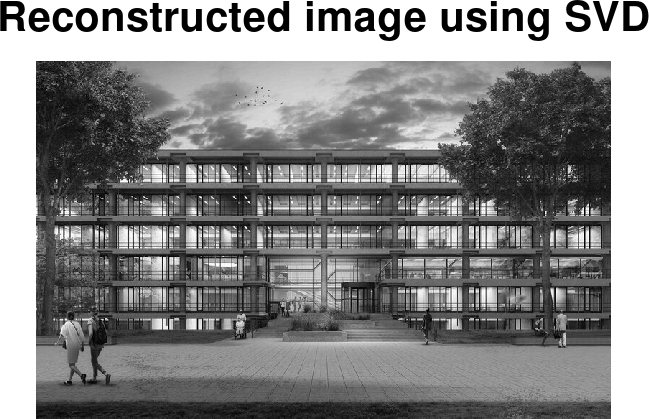

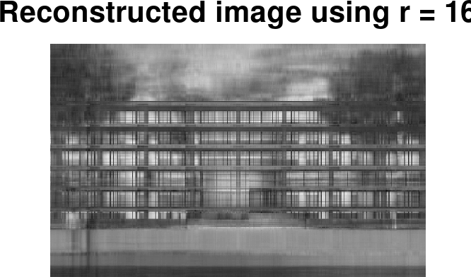
Data compression.

In a final step, we select only the $r$ most prominent columns of $U$ ($U_r$) and $V$ ($V_r$) that are associated with the largest singular values in $S$ ($S_r$).

14) What are the sizes of the matrices $U_r$, $S_r$, and $V_r$?

We can use some Matlab/Octave coding to shrink the matrices.

% set a low-rank value
r = 16;
% First r columns of U and V form Ur and Vr
Ur = U(:, 1:r)
Vr = V(:, 1:r)
% We should only keep the associated rows and columns of $S$ as well
% Such that we only keep the upper left r x r entries of S.
Sr = S(1:r, 1:r)
% Approximate the image using only $j$ singular vectors in both Ur and Vr
gs = Ur*Sr*Vr'; 
imshow(gs, []);

15) Try a few different values of $r$ and enjoy your low-rank approximations

16) What type of images would be well approximated with relatively small number of singular vectors?

Continue to the examples of week 5…