Applications of Linear Algebra and Multivariable Calculus

These pages present the example applications of the content covered in 8BA060: Linear algebra and multivariable calculus.

Week 1A: Fitting a curve to data points.

Consider three data points : $\{x, y\} = \{-1, 0\}, \{0,0\}$ and $\{0,1\}$. We fit a (non-linear!) polynomial relation of the form,

$$y(x) = ax^2 + bx + c.$$

Noting that the terms scale linearly with their respective unknowns ($a, b, c$). We can setup a system of linear equations,

$$\begin{pmatrix} 1 & -1 & 1\\0 & 0 & 1 \\ 1 & 1 & 1\end{pmatrix} \begin{pmatrix}a\\b\\c\end{pmatrix} = \begin{pmatrix}0\\0\\1\end{pmatrix}.$$

An echelon form of the augmented matrix is,

$$\begin{pmatrix}1&-1&1&0\\0&2&0&1\\0&0&1&0\end{pmatrix},$$

The solution ($a, b$ and $c$) for the parabola is thus; $c = 0$, $b = \frac{1}{2}$ and $a = \frac{1}{2}$,

$$y = \frac{1}{2}x^2 + \frac{1}{2}x.$$

We may visually verify in Octave/Matlab.

% Plot function for -2 < x < 2.
fplot (@(x) 0.5*x.^2 + 0.5*x, [-2, 2], "linewidth", 2, 'red');
hold on
% data points
scatter ([-1, 0, 1], [0, 0, 1], 'filled');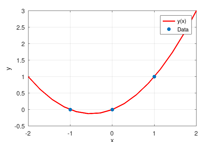

Polynomial fit with a free variable

Reconsider the three data points : $\{x, y\} = \{-1, 0\}, \{0,0\}$ and $\{0,1\}$. Lets try to fit a polynomial relation of the form,

$$y(x) = ax^3 + bx^2 + cx + d.$$

The linear system now reads,

$$\begin{pmatrix} -1 & 1 & -1 & 1\\0 &0 & 0 & 1 \\ 1&1 & 1 & 1\end{pmatrix} \begin{pmatrix}a\\b\\c\\d\end{pmatrix} = \begin{pmatrix}0\\0\\1\end{pmatrix},$$

with an echelon form of the augmented below having three (underlined) pivots for four unknowns, indicating one free variable.

$$\begin{pmatrix} \underline{1} & 1 & 1 & 1 & 1\\0 & \underline{2} & 0& 2 & 1 \\ 0&0 & 0 & \underline{1} & 0\end{pmatrix}.$$

The solution is: $d = 0$, the free variable: $c = t$, $b = \frac{1}{2}$ and $a = \frac{1}{2} - t$. For $t = \frac{1}{2}$, we obtain the previous parabolic solution. Using Octave, we may plot the solution for some some selected values of $t$.

fplot (@(x) 0.5*x.^3+0.5*x.^2, [-1.1, 1.1], 'linewidth', 2,'red')
hold on
fplot (@(x) x.^3+0.5*x.^2-0.5*x, [-1.1, 1.1], 'linewidth', 2,'green')
fplot (@(x) -0.5*x.^3+0.5*x.^2+1*x, [-1.1, 1.1], 'linewidth', 2,'magenta')
scatter([-1,0,1],[0,0,1], 'filled')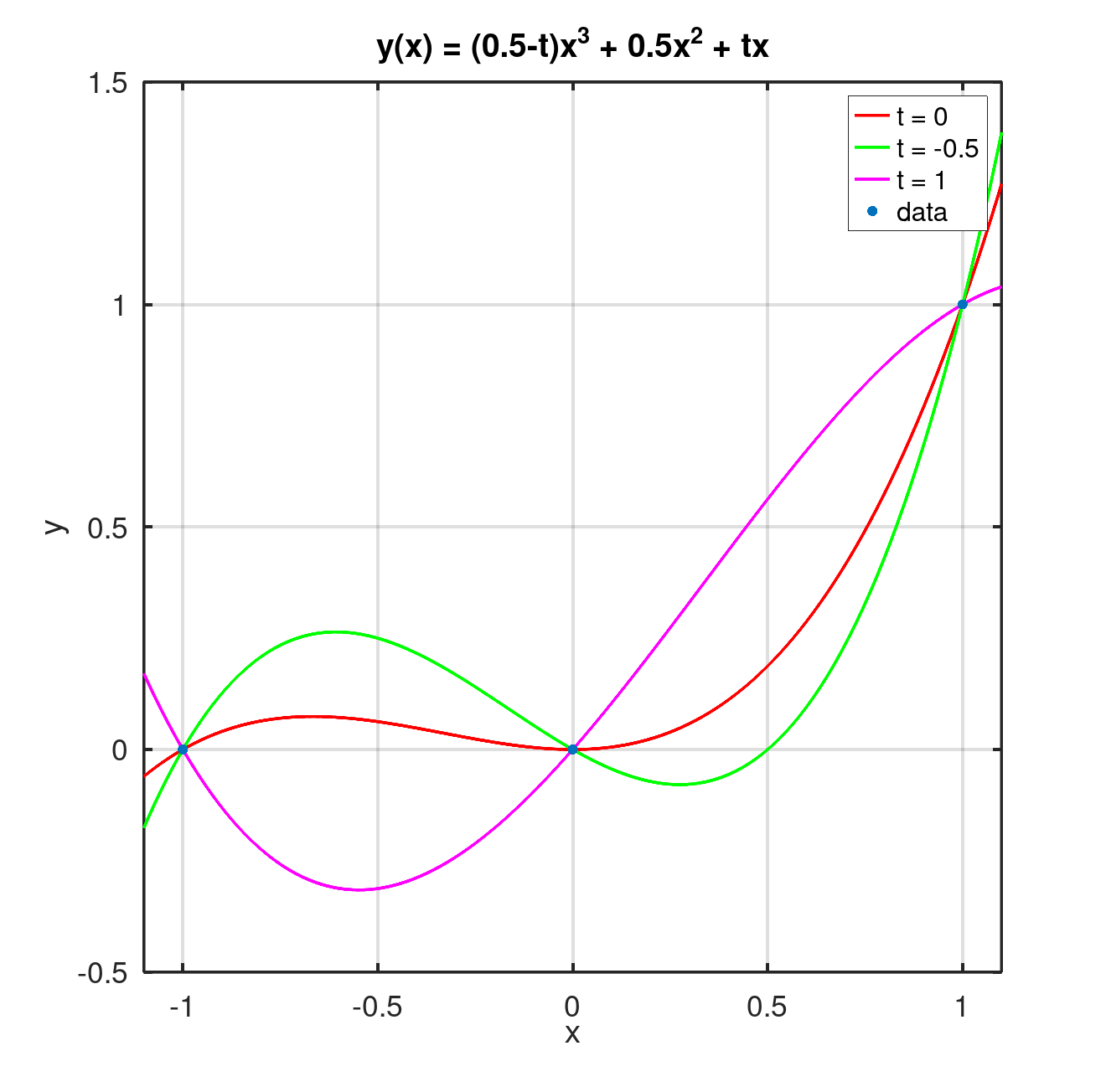

Thank you Gaussian elimination! for helping me to find these solutions.

Week 1B: Projection for computer graphics

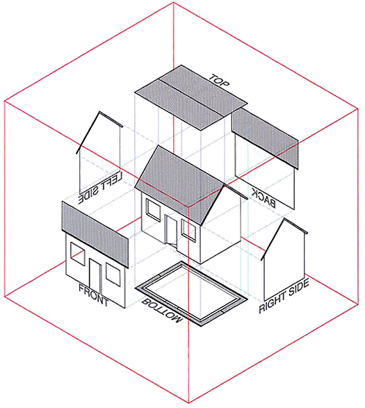
Parallel projection

Technical drawings are often presented using various “side views” of an object via a so-called orthographic projection. Here a point in three-dimensional (3D) space ($\mathbf{x} = \begin{pmatrix}x\\y\\z\end{pmatrix}$) is transferred to 2D screen-space coordinates, $\mathbf{p} = \begin{pmatrix}i\\j\end{pmatrix}$. A simple projection onto the $x-y$ plane is obtained by the linear map.

$$\mathbf{p}=\begin{pmatrix}1 & 0 & 0\\ 0 & 1 & 0\end{pmatrix}\mathbf{x}$$

Since the matrix is already in echelon form we can directly conclude that this is onto but not one-to-one. Its kernel is 1D and given by $t\begin{pmatrix}0\\0\\1\end{pmatrix}$, with $t \in \mathcal{R}$.

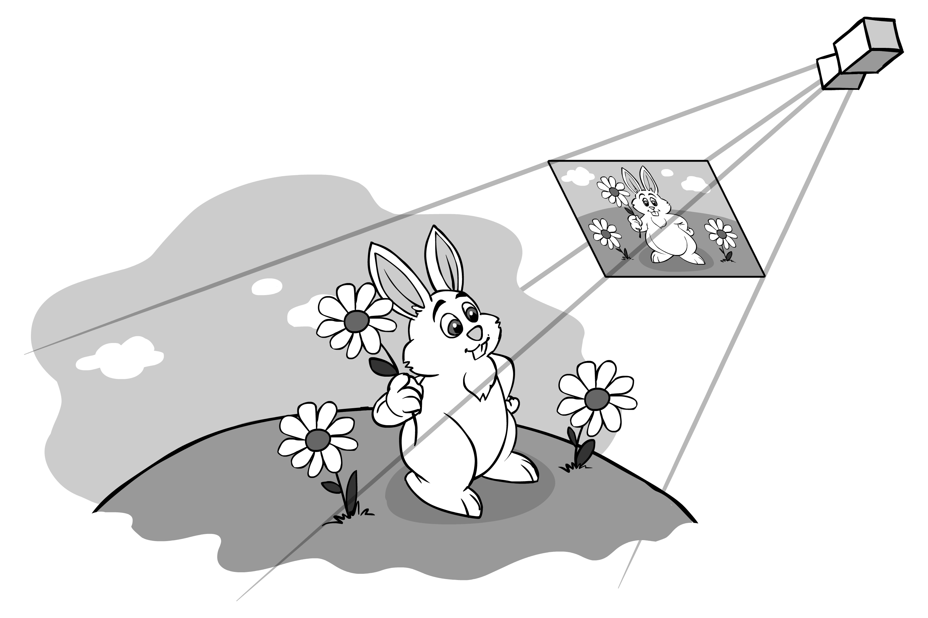
Perspective projection

A projection that better mimics our perception of the world is the so-called perspective projection. This is a linear map that is popular in graphics applications, and it is also given by a matrix transformation,

$$\begin{pmatrix}x'\\y'\\d\end{pmatrix} = \begin{pmatrix} A_{1,1}&A_{1,2}&A_{1,3}&t_x\\ A_{2,1}&A_{2,2}&A_{2,3}&t_y\\ A_{3,1}&A_{3,2}&A_{3,3}&t_z \end{pmatrix} \begin{pmatrix} x\\y\\z\\1\end{pmatrix}.$$

Here the $A_{m,n}$ coefficients encode the camera tilt angles and the $t_{x,y,z}$ is the translation of the camera. The final screen-space coordinates are then computed in a separate step, the so-called perspective division which causes far-away objects, with large distance $d$, to appear smaller,

$$i = \frac{x'}{d} \text{and } j = \frac{y'}{d},$$

or

$$\begin{pmatrix}i\\j\end{pmatrix} = \begin{pmatrix}\frac{1}{d}& 0 \\ 0 & \frac{1}{d}\end{pmatrix}\begin{pmatrix}x' \\y' \end{pmatrix}.$$

Thank you linear transformations! for all the nice computer graphics.

Continue to the examples of week 2…