Week 2A: Powers of the adjacency matrix

A social media website (like Linked-in) may suggest new friends/connections to connect with. It is possible to use matrix algebra in order to analyze the “proximity” of people in a complex network of connections. Consider an example network below of six people, lines (vertices) are drawn between persons (nodes) to indicate the existing connections.

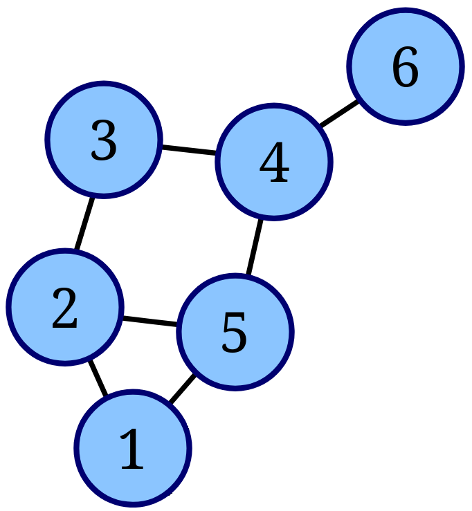
In a first step, we can characterize this network by its adjacency matrix $A$, a $6\times 6$ matrix where each element $A_{i,j}$ is either 1, if there is a connection between person $i$ and $j$ or 0, if there is not. As such, the adjacency matrix is a symmetric matrix. For the given graph above, the adjacency matrix is,

$$A = \begin{pmatrix} 0 & 1 & 0 & 0 & 1 & 0\\ 1 & 0 & 1 & 0 & 1 & 0\\ 0 & 1 & 0 & 1 & 0 & 0\\ 0 & 0 & 1 & 0 & 1 & 1\\ 1 & 1 & 0 & 1 & 0 & 0\\ 0 & 0 & 0 & 1 & 0 & 0\end{pmatrix}.$$

Put differently, $$A^1$ gives the number of paths of length 1 vertex between two persons. Lets say we broaden our scope and look at the number of paths between two persons that have a length of two vertices. This would mean counting the number of persons with which each of them has a connection of length 1. Say we want find out how many paths there are of length 2 between node 2 and 4 we can inspect the second and fourth row of the matrix,

$$\begin{pmatrix} &0 & 1 & 0 & 0 & 1 & 0\\ \rightarrow &1 & 0 & \underline{1} & 0 & \underline{1} & 0\\ &0 & 1 & 0 & 1 & 0 & 0\\ \rightarrow &0 & 0 & \underline{1} & 0 & \underline{1} & 1\\ &1 & 1 & 0 & 1 & 0 & 0\\ &0 & 0 & 0 & 1 & 0 & 0\end{pmatrix}.$$

The 3rd and 5th column have 1s on both rows, indicating a shared one-vertex connection, and thus there are two a possible paths from node 2 to 4 over two vertices (via node 3 or via node 5). Given the symmetry of the matrix we could have also compared the 2nd row to the 4th column instead of the 4th row.

$$\begin{pmatrix} & & & & \downarrow & &\\ &0 & 1 & 0 & 0 & 1 & 0\\ \rightarrow &1 & 0 & \underline{1} & 0 & \underline{1} & 0\\ &0 & 1 & 0 & \underline{1} & 0 & 0\\ &0 & 0 & 1 & 0 & 1 & 1\\ &1 & 1 & 0 & \underline{1} & 0 & 0\\ &0 & 0 & 0 & 1 & 0 & 0\end{pmatrix}.$$

You can now see that finding the number of 2-vertex paths is nothing but a row-column multiplication! As such, we can multiply $A$ with itself to get $A^2$, whose entries list the number of two-vertex connections between two nodes.

We can repeat the same argument for the 3-vertex connections encoded in $A^3$. For the given graph it is,

$$A^3 = \begin{pmatrix} 2&4& 2& 2& 4& 1\\ 4& 2& 5& 1& 6& 2\\ 2& 5& 0& 5& 1& 0\\ 2& 1& 5& 0& 6& 3\\ 4& 6& 1& 6& 2& 0\\ 1& 2& 0& 3& 0& 0\end{pmatrix}.$$

We see that this matrix is has non-zero diagonal entries. This corresponds to paths from a node to itself via three vertices. Such triangular paths always come in multiples of 6: For each node in a triangle there is a left and a right oriented path traversal. As such, we can sum the number of entries on the diagonal and divide by six to get the number of triangles in the netowrk. Using the trace ($\text{TR}(...)$) we can write for the number of triangles in a network ($N$),

$$N = \frac{\text{TR}(A^3)}{6}.$$

Thank you matrix algebra! for this neat fact.

Week 2A: Polynomial-line fitting revisited

Consider three data points $\{x,y\}$ with specific $x$ coordinates but with variable $y$ values given by $\{-1, y_{-1}\}, \{0, y_0\}$ and $\{1, y_1\}$. We can again try to fit a parabolic function,

$$y(x) = ax^2 + bx + c.$$

The matrix equation is,

$$A\begin{pmatrix}a\\b\\c\end{pmatrix} = \begin{pmatrix}1&-1&1\\ 0 & 0 &1\\ 1&1&1\end{pmatrix} \begin{pmatrix}a\\b\\c\end{pmatrix} = \begin{pmatrix}y_{-1}\\y_0\\y_1\end{pmatrix}.$$

or in short-hand notation,

$$A\mathbf{a} = \mathbf{y}$$

We can rewrite the equation by left-multiplication of the the matrix inverse,

$$\mathbf{a} = A^{-1}\mathbf{y}$$

Substituting the coefficients gives,

$$\begin{pmatrix}a\\b\\c\end{pmatrix} = \begin{pmatrix} \frac{1}{2}&-1&\frac{1}{2}\\ -\frac{1}{2}&0&\frac{1}{2}\\ 0&1&0 \end{pmatrix}\begin{pmatrix}y_{-1}\\y_0\\y_1\end{pmatrix}.$$

Instead of doing the Gaussian elimination procedure for every column vector $\mathbf{y}$, we plot find the polynomial coefficients ($\mathbf{a}$) using a simple matrix multiplication. We can apply this in Octave to generate the frames of the following movie.

A = [[1,-1,1];[0,0,1];[1,1,1]];
Ai = inv(A);

for i = 1:200
  t = 2.*pi*i/200
  y = [sin(t - 1); cos(t + 1); sin(2*t)];
  a = Ai*y;
  clf
  fplot (@(x) polyval(a, x), [-1.1, 1.1], 'linewidth', 2, 'red');
  hold on
  scatter ([-1, 0, 1], y, 'filled')
end

Finite difference

If we (can) assume that the data is part of some continuous signal (f(x)), it turns out to be quite OK to guess that locally this function can be approximated with a polynomial. Say we wish to find the second derivative at $x = 0$ we can differentiate our polynomial,

$$\frac{\mathrm{d}^2f}{\mathrm{d}x^2}\bigg\rvert_{x=0}\approx\frac{\mathrm{d}^2y}{\mathrm{d}x^2}\bigg\rvert_{x=0} = 2a.$$

By reading the matrix equation we can thus conclude that:

$$\frac{\mathrm{d}^2f}{\mathrm{d}x^2}\bigg\rvert_{x=0}\approx y_{-1}-2y_0+y_1$$

The process of using point-location values and estimating derivatives is part of the finite difference method, which is used for all kinds of numerical models in science and engineering.

Week 2B: The vector product (cross product)

Consider two vectors expressed with a Cartesian basis, $\vec{a} = a_x\vec{e}_x + a_y\vec{e}_y + a_z\vec{e}_z$ and $\vec{b} = b_x\vec{e}_x + b_y\vec{e}_y + b_z\vec{e}_z$. We can write their vector product $\vec{c} = \vec{a} \times \vec{b}$ as the determinant of a carefully constructed matrix,

$$\vec{c} = \vec{a} \times \vec{b} = \begin{vmatrix} \vec{e_x}&\vec{e_y}&\vec{e_z}\\ a_x&a_y&a_z\\ b_x&b_y&b_z\end{vmatrix} = (a_yb_z - a_zb_y)\vec{e}_y + (a_zb_x - a_xb_z)\vec{e}_y + (a_xb_y - a_yb_x)\vec{e}_z.$$

Thank you determinant for the convenient mnemonic!

Continue to the examples for the third week…