10. A Navier-Stokes problem solver

A time stepping function

We have arrived at the point where we can code our time-stepping function. This function of the form,

void advance_ns (double dt)

will advance the solution field (ux and uy) in time by a timestep dt. We already know that this will require the computation of the associated pressure field which we like to keep in between steps. So in ns.h we declare a global-scope field p[N][N] along with the velocity-component fields.

#include "common.h"
#include "poisson.h"

double ux[N][N], uy[N][N], p[N][N];

...

void projection (...) {
  ...
}

void advance_ns (double dt) {
}
...

As aforementioned, we will first compute the provisional velocity field. This is a separate update to the ux and uy scalar field according to the advection + diffusion equation. As such, we will first implement an advance_scalar () function that makes a time step for scalar fields.

...
void projection (...) {
   ...
}

void advance_scalar (double s[N][N], double ux[N][N], 
                     double uy[N][N], double kappa, double dt) {
  double ds_dt[N][N];
  tracer_advection (s, ux, uy, ds_dt);
  if (kappa > 0)
    diffusion (s, kappa, ds_dt);
  foreach()
    val(s, 0, 0) += dt*val(ds_dt, 0, 0);
}

void advance_ns (...) { 
...

We can use this to compute the provisional velocity field $\mathbf{u}^*$ in advance_ns() which we can not store in the original arrays, as they would be updated with different velocity fields.

...
void advance_ns (double dt) {
  // Declare and initialize and compute u_star
  double ux_star[N][N], uy_star[N][N];
  foreach() {
    val (ux_star, 0, 0) = val(ux, 0, 0);
    val (uy_star, 0, 0) = val(uy, 0, 0);
  }
  advance_scalar (ux_star, ux, uy, nu, dt);
  advance_scalar (uy_star, ux, uy, nu, dt);
}
...

To complete Chorin’s method, project $\mathbf{u}^*$ and update the solution.

  ...
  advance_scalar (uy_star, ux, uy, nu, dt);
  // Project and update
  projection (ux_star, uy_star, p, dt);
  foreach() {
    val (ux, 0, 0) = val(ux_star, 0, 0);
    val (uy, 0, 0) = val(uy_star, 0, 0);
  }
}
...

Two tests

We should now test the combined functions of our code. A difficulty with the non-linear Navier-Stokes equations is that finding non-trivial solutions is hard, which limits the ability to test a solver. Here we will consider two flow solutions, one will be investigated qualitatively, the other quantitatively.

The Lamb-Chaplygin dipole

I am proud to say that I lead authorship for the Wikipedia page on the Lamb-Chaplygin dipole. Quoting myself,

The Lamb–Chaplygin dipole model is a mathematical description for a particular inviscid and steady dipolar vortex flow. It is a non-trivial solution to the two-dimensional Euler [Navier-Stokes] equations. The model is named after Horace Lamb and Sergey Alexeyevich Chaplygin, who independently discovered this flow structure.¹

Here we test if our solver can represent this steady solution. We will use the stream function ($\psi$) to initialize the flow field. Which are related by,

$$u_x = \frac{\partial \psi}{\partial y}, u_y = -\frac{\partial \psi}{\partial x}.$$

The stream function for the Lamb-Chaplygin dipole in cylindrical coordinates ($r, \theta$) reads,

$$\begin{align} \psi = \begin{cases} U\left(\frac{-2 J_{1}(kr)}{kJ_{0}(kR)} + r\right)\mathrm{sin}(\theta) , & \text{for } r < R, \\ U\frac{R^2}{r}\mathrm{sin}(\theta), & \text{for } r \geq R, \end {cases} \end{align}$$

However, this formulation is based on an infinitely large domain size. As such, we will focus on the (2D scalar) vorticity ($\omega = -\frac{\partial u_x}{\partial y} + \frac{\partial u_y}{\partial x}$) distribution,

$$\begin{align} \omega = \begin{cases} kU\left(\frac{-2 J_{1}(kr)}{J_{0}(kR)}\right)\mathrm{sin}(\theta) , & \text{for } r < R, \\ 0, & \text{for } r \geq R, \end {cases} \end{align}$$

where $R$ is the size of the circular dipole, $U$ is it’s translation velocity, $J_0$ and $J_1$ are the zeroth and first Bessel functions of the first kind, and the value for $k$ is such that $kR = 3.8317$, the first non-trivial zero of the first Bessel function of the first kind. We can compute a suitable stream function via the (Poisson) relation,

$$\nabla^2 \psi = -\omega,$$

which can then be used to compute $\mathbf{u}(t = 0)$.

Lets code it up in lamb.c. We start by carefully implementing the vorticity field ($\omega$, omega) , solving for $\psi$ (psi) and computing the initial velocity field.

#include "ns.h"
#include "visual.h"
#define RAD (sqrt(sq(x) + sq(y)))
#define SIN_THETA (RAD > 0 ? y/RAD : 0)
double U = 1, R = 1;

int main () {
  L0 = 15;
  X0 = Y0 = -L0/2.;
  double k = 3.8317/R;
  double omega[N][N], psi[N][N]; 
  foreach() {
    if (RAD < R) 
      val (omega, 0, 0) = -k*U*(-2*j1(k*RAD))/(j0(k*R))*SIN_THETA;
    else 
      val (omega, 0, 0) = 0;
    val (psi, 0, 0) = 0;
  }
  max_sweeps = 10000;
  poisson (psi, omega);
  // Compute inital velocity field
  foreach() {
    val (ux, 0, 0) =  (val(psi, 0, 1) - val(psi, 0, -1))/(2*Delta) - U;
    val (uy, 0, 0) = -(val(psi, 1, 0) - val(psi, -1, 0))/(2*Delta);
  }
}

We should visually inspect the initialization by looking at the velocity components, and check if the vorticity in still entirely concentrated in a circular region. Hence we diagnose the vorticity field, reusing the omega field.

 ...
     val (uy, 0, 0) = -(val(psi, 1, 0) - val(psi, -1, 0))/(2*Delta);
  }
  output_ppm (ux,"ux.ppm", -U, U);
  output_ppm (uy,"uy.ppm", -U, U);
  foreach() {
    val(omega, 0, 0) = -(val(ux, 0, 1) - val(ux, 0, -1))/(2*Delta);
    val(omega, 0, 0) += (val(uy, 1, 0) - val(uy, -1, 0))/(2*Delta);
  }
  output_ppm (omega, "vort.ppm", -U*k, U*k);
}

Compile, run and inspect,

$ gcc -DN=300 lamb.c -lm
$ ./a.out
# Warning: max res = 0.00315803 is greather than its tolerance (0.0001)
$ convert ux.ppm uy.ppm vort.ppm +append xyo.png

After the inevitable syntax-error fixes, we can inspect xyo.png.

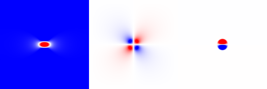
This looks good and we can setup a time loop,

...
  output_ppm (omega, "vort.ppm", -U*k, U*k);

  // Time loop
  int iter = 0; 
  double t_end = 2;
  for (t = 0; t < t_end; t += dt) {
    printf ("# i = %d, t = %g\n", iter, t);
    dt = dt_next(t_end);
    advance_ns (dt);
    iter++;
  }
}

To verify if our solution remained steady, we can output the vorticity field at the end of the simulation,

    ...
    iter++;
  }
  // Output vorticity field
  foreach() {
    val(omega, 0, 0) = -(val(ux, 0, 1) - val(ux, 0, -1))/(2*Delta);
    val(omega, 0, 0) += (val(uy, 1, 0) - val(uy, -1, 0))/(2*Delta);
  }
  char fname[99];
  sprintf (fname, "o-%d.ppm", N);
  output_ppm (omega, fname, -U*k, U*k);
}

Compile run and check,

$ gcc -O3 lamb.c -lm
$ ./a.out 
...
# i = 24, t = 1.7463
# i = 25, t = 1.83109
# i = 26, t = 1.91627

After a second or two of simulation I increase the image size a bit and add an annotation whilst converting it to a .png to show here.

$ convert o-100.ppm -resize 300x300 -pointsize 30\
              -annotate +100+70 'N = 100' o-100.png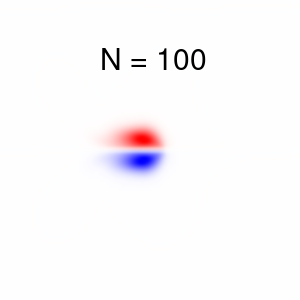

The vortex structure seems to have survived(!) but in a deformed state. We should also check if this deformation at least decreases if we increase the accuracy of our computations.

$ gcc -DN=200 -O3 lamb.c -lm
$ ./a.out
...
$ gcc -DN=400 -O3 lamb.c -lm
$ ./a.out
...

Then we prepare our comparison (I did not put the ampersands ($) so the block below maybe copied and pasted).

convert o-200.ppm -resize 300x300 -pointsize 30\
              -annotate +100+70 'N = 200' o-200.png
convert o-400.ppm -resize 300x300 -pointsize 30\
              -annotate +100+70 'N = 400' o-400.png
convert vort.ppm -resize 300x300 -pointsize 30\
              -annotate +80+70 'Reference' vort.png
convert o-100.png o-200.png +append o-top.png
convert o-400.png vort.png +append o-bottom.png
convert o-top.png o-bottom.png -append o-2x2.png

The resulting image (o-2x2.png) is shown below,

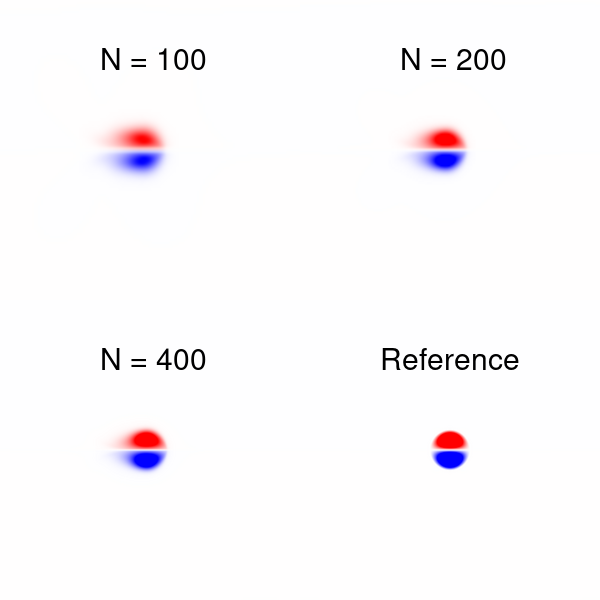
I consider this a pass. Notice that this test is far from perfect, it is unclear what the effects of our finite L0 and the periodic boundaries are. But I do know (from experience) that this test is more critical than the qualitative test below.

Taylor-Green vortices

We will adhere to the tradition of testing new flow solvers against the Solution of Taylor and Green. On a periodic domain of size $2\pi \times 2\pi$,

$$u_x = \cos(x)\sin(y)e^{-2\nu*t},$$ $$u_y = -\cos(y)\sin(x)e^{-2\nu*t}.$$

We will make it more interesting by evaluating it in a moving frame of reference. We will do a convergence test for the $L_2$ error. Using tg.c,

#include "ns.h"

#define UX (cos(x)*sin(y)*exp(-2*nu*t) + 1)
#define UY (-cos(y)*sin(x)*exp(-2*nu*t) + 1)

int main() {
  L0 = 2*3.14159265;
  nu = 0.1; 
  // Initialize
  foreach() {
    val(ux, 0, 0) = UX;
    val(uy, 0, 0) = UY;
  }
  // Solve until t = 2*pi
  double t_end = L0;
  int iter = 0;
  for (t = 0; t < t_end; t += dt) {
    dt = dt_next(t_end);
    advance_ns (dt);
    iter++;
  }
  // Compute L2 for ux and uy combined
  double L2 = 0;
  foreach() {
    L2 += sq(Delta)*sq(val(ux, 0, 0) - UX);
    L2 += sq(Delta)*sq(val(uy, 0, 0) - UY);
  }
  printf ("%d %d %g %g\n", N, iter, t, L2);
}

Compile and compare the results

$ gcc -O3 tg.c -lm
$ ./a.out
100 1592 6.28319 0.18054
$ gcc -O3 -DN=200 tg.c -lm
$ ./a.out
200 6367 6.28319 0.0581281
$ gcc -O3 -DN=400 tg.c -lm
$ ./a.out 
$ 400 25465 6.28319 0.0166069

Convergence looks OK since $\frac{0.18}{0.058} \approx \frac{0.058}{0.016} \approx 3.3$, which is a quite healthy. Given the the number of time steps has increases by a factor of 4 with doubling resolution indicates that the viscous term is most stringent for our time stepping stability. The factor 3.3 is a mix of the accuracy of the dominant diffusion term (second order accuracy would give a reduction factor of $\left(\frac{400}{200}\right)^2 = 4$) and the first-order accuracy for the advection term ( $\left(\frac{400}{200}\right)^1 = 2$). In this case $2 + 4 \approx 3.3$.

The patient among us may want to push a bit more a do $N = 800$,

$ gcc -O3 -DN=800 tg.c -lm
$ ./a.out
Segmentation fault

This is an error raised by our operating system that does not allow to allocate so much memory for our fields on the stack. We could tell it to give us more.

$ ulimit -s
8192
// i.e in Kbytes default
$ su 
// Enter password 
# ulimit -s 100000
# ./a.out

This is not really a good solution. Using malloc is! But this would go against a core design principle of our solver, namely coding simplicity. Notice that the high-resolution runs are prohibitively expensive anyway.

Congratulations!

You have wrote a Navier-Stokes equation solver and It is therefore almost time to have some flow-related fun. First, we should make small improvements to the functionality of our code before we can really show-off some flow cases in a gallery. Lets code up some more function and an improved user interface.